how to create a drop down list in google sheets

Download PC Repair Tool to quickly find & fix Windows errors automatically

Google Sheets is a free web-based application and a popular alternative to Microsoft Excel. The tool allows to easily create, update, and modify spreadsheets. It serves as an excellent collaborative tool allowing you to add as many people as you want and edit Google Sheets with others at the same time. The online tool enables you to work jointly in real-time on a project in the same spreadsheet irrespective of wherever you are located. To collaborate on Google Sheets one has to simply click a Share button and there you are allowing your friends, colleagues, or family to edit your spreadsheet.

When working on a shared Google Spreadsheet, you may want other users to enter only restricted data within its cells. To avoid others entering wrong values within cells, you may want to add a graphical control element like the drop-down menu which is similar to a list box that would allow people to enter only those values available from a given list. Apart from that, the drop-down list serves as a smart and more efficient method to enter data.

That being said, a drop-down list or a pulldown menu is a streamlined way to ensure that people fill only the values into your cells in the exact same manner as your expecting. Like Excel, Google Sheets allows you to easily create a drop-down menu to your Sheets. Additionally, it enables you to make partial changes to the drop-down list in case you want to modify the selection list in the cells. In this article, we explain in detail how to create a drop-down menu in Google Sheets and modify the same.

Create a drop-down menu in Google Sheets

Launch Google Sheets

Open a new spreadsheet or open an existing spreadsheet file.

Select a cell where you want to create a drop-down list. You can also select a group of cells, an entire column, or a row.

Navigate to Sheets menu and click on the option Data.

create and modify a drop-down list in Google Sheets

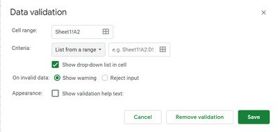
Select Data Validation from the drop-down menu. A Data Validation window pops up with several options to customize.

The first field in the Data Validation window is the Cell range which is automatically filled based on the selected cells. You can change the range to a new value by simply clicking on a table icon in the Cell Range field.

The second field in the Data Validation window is the Criteria which has a list of various options in its own drop-down menu. The Criteria contains options like List from a range, List of items, Number, Text, and Date.

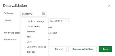
List from a range: This option allows you to create a list of values that have been retrieved from different sheets or the list of values from different cells on the same sheet.
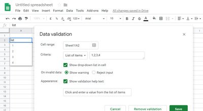
List of items: This allows us to create a list of text values. They are entered in the edit field separated by commas.
Number: This Option doesn't create a drop-down list instead makes sure that the entry to the drop-down menu falls within a specific numeric range.
Text: This Option doesn't create a drop-down list instead makes sure that the entry is in a proper textual format.
Date: This Option doesn't create a drop-down list instead makes sure if the date entered is valid or comes in a certain range.
Custom Formula is: This option does not create a drop-down list instead makes sure the selected cell uses a user-specified formula.

Once the data that is to be included in the list is entered, select the option Show dropdown list in cell. Selecting this option ensures that the values appear in the cells.

You can also choose what has to be done when someone enters an invalid data which is not present on the list by selecting the options with a radio button. You can choose to have either Show warning option or Reject input option on invalid data. The Reject Input option doesn't allow you to enter any value which is not present on your drop-down list. On the other hand, Show warning option allows you to enter the invalid data which is not on your list but displays the warning message in the sheet.

The last option in the setting window is the Appearance. This option gives a hint to the user on what values or data they can enter in the cells. To activate this assistant, select the option Show validation help text beside the Appearance field. After you select the option, type the instructions that want to give people about what values they can choose within the cell range.

Click Save to apply the changes.

Edit the drop-down list in Google Sheets

To add more values to the list or remove items from the drop-down menu follow the below steps

Navigate to Data and select Data validation from the drop-down menu.

Select the cells and change the items in the entry.

Click Save to apply changes.

That's all.

Shiwangi loves to dabble with and write about computers. Creating a System Restore Point first before installing new software, and being careful about any third-party offers while installing freeware is recommended.